Exact Diagonalization: The Bose–Hubbard Model as an Example

This is an English translation of the Chinese original, first published on 20 July 2025 (use the 中文 button in the menu to read it). The translation was prepared with the assistance of Claude Opus 5.5 (Anthropic).

This post follows the exact diagonalization method in the paper by J M Zhang and R X Dong. Using the Bose–Hubbard model as an example, it shows how to construct the corresponding Hamiltonian. The code is given in MATLAB.

The Bose–Hubbard model

The Bose–Hubbard model is the model with the following Hamiltonian:

\[\begin{equation} \hat{H}=-t\sum_{\langle ij\rangle}(a_{i}^{\dagger}a_{j}+a_{j}^{\dagger}a_{i})+\frac{U}{2}\sum_{i=1}^{M}\hat{n}_{i}(\hat{n}_{i}-1) \end{equation}\]

Here \(a_{i}(a_{i}^{\dagger})\) is the bosonic operator that annihilates (creates) a particle on site \(i\), and the number operator \(\hat{n}_{i}=a_{i}^{\dagger}a_{i}\) counts the particles on site \(i\). Because the model is bosonic, more than two particles can share a site. We consider a finite one-dimensional lattice with \(M\) sites in total. If the total number of atoms is \(N\), the dimension of the full Hilbert space follows from the stars-and-bars argument:

\[\begin{equation} D=\frac{(N+M-1)!}{N!(M-1)!} \end{equation}\]

This dimension grows exponentially. Symmetries could be used to reduce the number of basis states, but here we only consider a basic numerical method, so no symmetry analysis is done.

The main content of this post follows the reference^[1], which gives an algorithm for building the Bose–Hubbard model for exact diagonalization. For simplicity, we use periodic boundary conditions.

Constructing the basis

We need to consider every way of distributing \(N\) particles over \(M\) sites. Loops can generate the basis, but relatively slowly. In fact, for Fock states we can define a lexicographic order to arrange all the basis states.

Given two Fock basis vectors \(|n_{1},n_{2},\cdots,n_{M}\rangle\) and \(|\bar{n}_{1},\bar{n}_{2},\cdots,\bar{n}_{M}\rangle\), there must be an index \(1\le k\le M-1\) such that \(n_{i}=\bar{n}_{i}\) for \(1\le i\le M-1\), while \(n_{k}\neq \bar{n}_{k}\). We define that if \(n_{k}\ge\bar{n}_{k}\) (\(n_{k}\le\bar{n}_{k}\)), the vector \(|n_{1},n_{2},\cdots,n_{M}\rangle\) is superior (inferior) to the vector \(|\bar{n}_{1},\bar{n}_{2},\cdots,\bar{n}_{M}\rangle\). One can show that this defines a total order on the basis vectors. Clearly \(|N,0,\cdots,0\rangle\) is superior to all other basis vectors, and \(|0,0,\cdots,N\rangle\) is inferior to all of them.

With this total order, we can start from \(|N,0,\cdots,0\rangle\) and generate all the other occupation-number basis states in descending order. Given a basis vector \(|n_{1},n_{2},\cdots,n_{M}\rangle\) with \(n_{m}<N\), the rule for generating the next vector below it is as follows.

Let \(n_{k}\neq0\) with \(n_{i}=0\) for all \(k+1\le i\le M-1\). Then the next basis vector \(|\bar{n}_{1},\bar{n}_{2},\cdots,\bar{n}_{M}\rangle\) satisfies:

• \(\bar{n}_{i}=n_{i}\) for \(1\le i\le k-1\);
• \(\bar{n}_{k}=n_{k}-1\);
• \(\bar{n}_{k+1}=N-\sum_{i=1}^{k}\bar{n}_{i}\), and \(\bar{n}_{i}=0\) for \(i\ge k+2\).

% Initialize the basis through cell
Basis = repmat({zeros(1, N_Sites)}, Dimension, 1);
% Set the first basis as (N, 0, 0...)
Basis{1}(1) = N_atoms;
% Basis Generation
for ii = 2: Dimension
    % find the index of k
    Count = find(Basis{ii-1}(1:end-1)~=0, 1, 'last');
    temp = Basis{ii-1};
    if Count <= N_Sites - 1
        if temp(Count) ~= 0 && ~any(temp(Count+1:end-1))
            Basis{ii}(1:Count-1) = Basis{ii-1}(1:Count-1);
            Basis{ii}(Count) = Basis{ii-1}(Count) - 1;
        Basis{ii}(Count + 1) = N_atoms - sum(Basis{ii}(1:Count));
    end
    end
end
Basis = cell2mat(Basis);

This produces all the basis states. The resulting Basis is a \(D\times M\) matrix: each row is one basis state, and each component of a row is the occupation number of that site.

Constructing the Hamiltonian

Once the basis is built, we can start constructing the matrix elements of the Hamiltonian:

\[\begin{equation} H_{uv}=\langle u|H|v\rangle \end{equation}\]

The Hamiltonian we need is usually a sparse matrix, so we only have to find its nonzero elements. The Bose–Hubbard Hamiltonian has two parts: the kinetic hopping term \(H_{\text{kin}}\) and the interaction term \(H_{\text{int}}\). The interaction term is diagonal in the occupation-number representation, so the main problem is building the hopping term.

The direct idea is to loop over all pairs of basis vectors. This of course works, but once the Hilbert space dimension reaches millions, sweeping through the whole Hamiltonian matrix takes an extremely long time. The kinetic part of the Hamiltonian has the form \(a_{i}^{\dagger}a_{j}\), and these hoppings are always between nearest neighbours (for example, in one dimension with \(M>3\) sites, site 2 has two hoppings, \(2\to 3\) and \(2\to1\)). So for \(M\) sites there are at most \(2M\) hopping terms. A simpler approach is therefore: first sort the basis; then, given the basis vector \(|v\rangle\) belonging to column \(v\) of the Hamiltonian, find the basis states produced when the kinetic term acts on it, and multiply by the hopping coefficients. This gives the nonzero entries, and the positions of those basis states give the row indices of the nonzero elements. For example, take 5 sites and 3 particles. Given the basis state \(|0,3,0,0,0\rangle\), its two hoppings give \(|1,2,0,0,0\rangle\) and \(|0,2,1,0,0\rangle\), so the nonzero rows in column \(v\) of the Hamiltonian are the positions of these two basis states. Looping over all columns then gives the kinetic part of the Hamiltonian. With this method, the problem becomes one of finding where the nonzero vectors produced by the Hamiltonian sit in the ordered basis, which gives the row and column indices of the Hamiltonian.

To match the resulting vectors, rather than comparing values one by one, we can use a hashing technique to find them faster. Simply put, hashing assigns each basis vector a tag, so to check whether two vectors are the same we only need to check whether their tags agree.

Since we already defined a lexicographic order when generating the basis, we can use it further to define a tag function. One possible choice is

\[\begin{equation} T(|v\rangle)=\sum_{i=1}^{M}\sqrt{p_{i}}v_{i} \end{equation}\]

where \(p_{i}\) can be the \(i\)-th prime. MATLAB's prime function is not fast at generating primes, so, following the paper^[1], one can simply use \(p_{i}=100i+3\).

Once the basis is numbered, we can also sort the basis vectors by tag value for faster lookup. Binary search then finds any vector among the \(D\) basis vectors in only \(\log_{2}D\) steps.

Tags = Basis * sqrt(100 * (1: N_Sites) + 3)';
% Sort the Tag function
[Tags, ind] = sort(Tags);

In the end we only need the rows, columns and values of the nonzero elements, and the sparse command builds the kinetic part of the Hamiltonian. The corresponding MATLAB code is:

for ii = 1: Dimension
    ind_nonzero = find(Basis(ii,:));
    for jj = 1: length(ind_nonzero)
        % Nearest hopping
        % Left hopping matrix element
        temp = Basis(ii,:);
        temp(ind_nonzero(jj)) = temp(ind_nonzero(jj)) - 1;
        temp_site = ind_nonzero(jj) - 1;
        if temp_site == 0
            temp_site = N_Sites;
        end
        temp(temp_site) = temp(temp_site) + 1;
        temp_Tag = temp * Tag_function(N_Sites)';
        col(Count) = ii;
        row(Count) = ind(abs(Tags - temp_Tag) < Accuracy);
        val(Count) = sqrt(Basis(ii,ind_nonzero(jj)) * (Basis(ii, temp_site)+1));
        Count = Count + 1;
        
        % Right hopping matrix element
        temp = Basis(ii,:);
        temp(ind_nonzero(jj)) = temp(ind_nonzero(jj)) - 1;
        temp_site = ind_nonzero(jj) + 1;
        if temp_site == N_Sites + 1
            temp_site = 1;
        end
        temp(temp_site) = temp(temp_site) + 1;
        temp_Tag = temp * Tag_function(N_Sites)';
        col(Count) = ii;
        row(Count) = ind(abs(Tags - temp_Tag) < Accuracy);
        val(Count) = sqrt(Basis(ii,ind_nonzero(jj)) * (Basis(ii, temp_site)+1));
        Count = Count + 1;
    end
end
H_kinetic = sparse(row, col, val);

The approach here is: take a basis vector \(|v\rangle\) as the column index; loop only over the sites with nonzero occupation; for each, consider hopping to the right and to the left, find the index of the resulting vector and record it as the row index, and record the value produced by the hop. Finally, the sparse command builds the matrix.

Note that in a many-particle system

\[\begin{equation} a_{i}^{\dagger}a_{j}|v\rangle=\sqrt{(v_{i}+1)v_{j}}|\cdots,v_{i}+1,\cdots v_{j}-1,\cdots\rangle \end{equation}\]

which brings in extra particle-number factors.

Last comes the diagonal interaction part, which takes a single line:

H_interaction = spdiags(sum(Basis .* (Basis - (Basis>0)),2), 0, Dimension, Dimension);

Putting the pieces together gives the Hamiltonian of the Bose–Hubbard model:

H = -t * H_kinetic + U/2 * H_interaction;
spy(H)

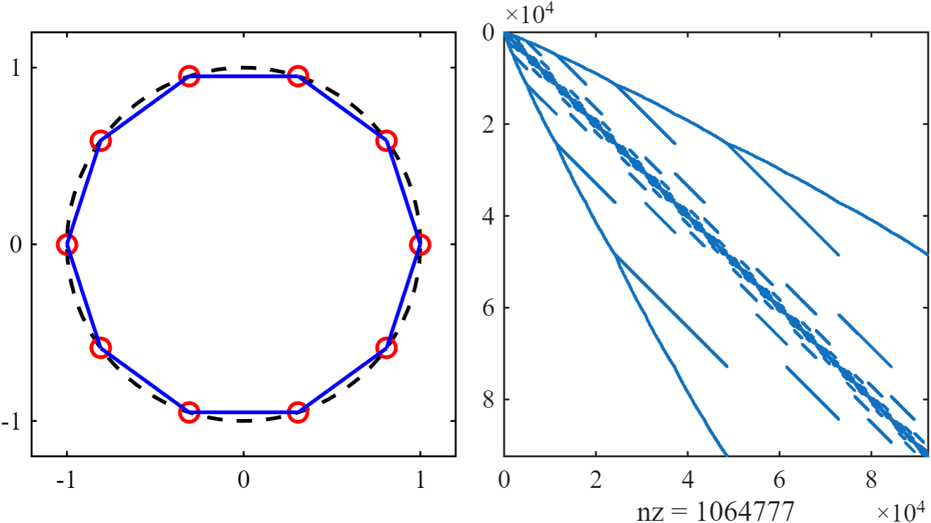
Left: the lattice for M=10 and N=10. Right: the sparsity pattern of the corresponding Hamiltonian.

---

1. 1.J M Zhang and R X Dong. Exact diagonalization: The Bose–Hubbard model as an example. European Journal of Physics, 31(3):591–602, May 2010. ↩︎